Using COUNTIF Function in Google Sheets to Describe Categorical Variable

Many times when we analyze data, we have some textual, or categorical variables. For example, we can have small, medium and big. Or we can have gender as male and female. Many times our data can use Yes and No as an answer. So, it becomes problematic to analyze such categorical data because we can not perform arithmetic on them. For this purpose COUNTIF function in Google Sheets can be very useful.

When it comes to the categorical variable, there are only a few possibilities for describing them. We can analyze them with counting. For example, we can count the number of categories. Many categorical variables have only two values as Male and Female for gender. Other variables as City and Region can have more than two categories.

I need to mention that some categorical variable can be coded numerically. For example, if we have data in the form of small, medium and big, we can code them as 1, 2 and 3. Or if you have totally disagree, disagree, agree, and totally agree we can code them as 0, 1, 2 and 3. Even we code some of the categorical variables, still, it is better to have additional text descriptions of these categories that can be useful later when we will make statistical reports.

Counting of Categorical variable

When you know the number of categories and their names, the only thing we can do is to start counting the number of observations in each category. We can make the number counts, or in some cases for the better description of the data, we can use percentages.

For example, if there are 10000 rows in our data set, with counting, we will have the new table with 4960 males and 5040 females, or also we can calculate and show that 49,6% of the observations are males and 50,4% are females. For me, it is useful to calculate the counts in both, numbers and percentage. And, when you have the counts, you can quickly display them graphically.

For this calculations, we will use the same data set as we used in the previous article related to the UNIQUE function in Google Sheets.

As you can see from the data, the Region, Sales Team, Customer ID, Gender, Marital Status, City and Product Family are all categorical variables. For easier calculations, I will make the named range for all my categorical variables: Region, Sales Team, Customer ID, Gender, Marital Status, City, and Product Family. I already describe how you can make named ranges in Google Sheets when I write about the VLOOKUP function.

Now everything is ready for our analysis and use of COUNTIF function.

Using the COUNTIF Function in Google Sheets (COUNTIF Formula Example)

The first thing I will do now is open the new sheet in Google Sheets. It will be easier to make the analysis.

The first calculations we will make is about the Region data. Now we will need to pull out all the unique variables in the Region column. We will do this using the UNIQUE function.

The COUNTIF syntax is COUNTIF(range, criterion) that returns a conditional count across a range and where the range is the data that we want to make counting against the specific criterion and the criterion is the pattern or test we want to apply to the range.

Steps You Need to Take to Calculate Using COUNTIF function in Google Sheets

1. Click on A1 cell in the new sheet.
2. Write the formula: =UNIQUE(Region) – the Region in the formula is our already defined name range.
3. The Google Sheet will give us all the unique values from the Region range in the A column.
4. Write the Count as a title for the B column.
5. Click on B2 cell.
6. Write the following formula: =COUNTIF(Region,A2). The Range in the formula is our already defined name range, while A2 is the criterion that tells Google Sheet to look in the Region range and count all data for the value in the A2 cell. The result is 215 times North-East region is found in the Region range.
7. Copy B2 cell and paste into the B3:B8. Now we will have counts for all regions.
8. Usually, I want to check if everything is ok using the total number of variables. I will make this with the help of the SUM function, clicking on the B9 cell and using the following formula: =SUM(B2:B8). The result is 1090 that is the number of rows in our data set.

Now I will have this table as a result of our analysis.

Steps You Need to Take to Calculate Percentages

To get the percentages in column C, each count from column B is divided by the total number of observations in cell B9.

1. Click on C2 cell.
2. Select the column C and format it as a Percent.
3. Write the formula: =B2/$B$9 (We use $ sign to tell Google Sheets to use B9 value for all calculations when we copy the B2 cell and paste in the B3:B8 as next step)
4. Copy the B2 cell and paste in the B3:B8.
5. As a check, it is useful to sum these percentages and check if the sum is 100%. So, in the C9 I will put this formula: =SUM(C2:C8)

Now the table will look like this:

Continue with the same steps for all other categorical variables. Here is how it looks when I made all the calculations for all categorical variables:

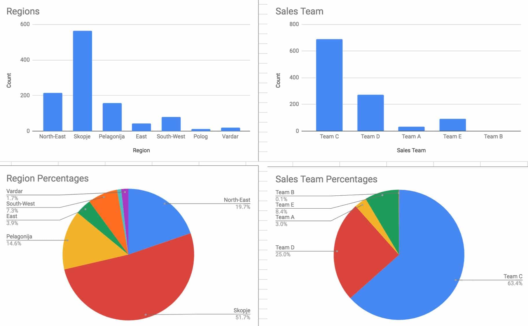
As you can see from the results now we have interesting results from the analysis of this data. Our company has the worst results in the Polog and Vardar region, or that the worst team is Team B with 0,09% of all transactions in the analyzed period of time.

Additionally, having these new tables, we can easily make charts for the better understanding of the analysis result. Here is an example of charts related to the implementation of COUNTIF function on Region and Sales Team. One chart is related to counts and another for percentages.

You need to have in mind that the COUNTIF function is related only to counting. In the analysis that we make here, we don’t take into considerations the revenue from each transaction, but only how much transactions we make. For example, if we analyze regions, we can have 100 transactions in one region but all of them below $100. On the other hand, we can have another region with only 20 transactions but all of them more than $1000 in revenue. So, we can not still make the conclusion about the best regions if we don’t analyze the additional variable as revenue in this case.

COUNTIF Greater Than and Less Than Zero

Sometimes you will want to count the number of data in the specific table with values greater or less than zero. In such a case you can use again the COUNTIF function in Google Sheets.

For example, you have the table with different positive and negative numbers and you want to see how much of them are positive and how much of them are negative. So, the COUNTIF function will do the job for you.

So, the using the COUNTIF syntax in this example, we will get the result that in the given data set there are 8 negative numbers.

If we use the same COUNTIF syntax for the same data set, but for positive numbers where criterion will be “>0” we will get the result for 13 positive numbers.

So, you have different options to use the COUNTIF function in Google Sheets. You only need the data range and criterion that will be used for counting.

If you want more tips and tricks check our category for analytics using Google Sheets category.